Stage 3 · Object detection

Assembling a versioned YOLO dataset by query from MySQL, fine-tuning a fish detector, and registering it in MLflow.

Govinda Lienart · AquaMind · Stage 3

prepare_dataset.py · DVC · YOLOv8s on Kaggle · MLflow Model Registry · 260 frames · mAP50 0.61

Abstract

Stage 3 turns the labelled rows stored in Stage 2 into a trained detector, in three steps. prepare_dataset.py selects the annotated frames of a chosen list of labelling batches, splits them 80/20 into training and validation sets under a fixed random seed, and writes them out in the folder layout YOLO expects, together with a dataset card recording exactly which batches, videos and code commit produced it. The dataset is versioned with DVC and fine-tuned on a Kaggle GPU, and log_artifact_mlflow.py logs the run and registers the resulting weights in the MLflow Model Registry under the alias @baseline; Stage 5 retrains it and promotes the better version to @champion. Trained on 260 ordinary frames from three videos, the baseline reaches mAP50 0.61 and mAP50-95 0.24 on its validation split. It finds most fish, but confuses fish and reflections in both directions and draws loose boxes. Later stages load it by alias, not by file path, and its measured failure modes are the starting point for the targeted labelling in Stage 5.

Introduction

Every measurement AquaMind makes, from how far a fish swims to when it chases another, begins with one question asked of every frame: where are the fish? Answering it is the job of an object detector, a model that takes a single image and returns a box around each object it recognises, the object’s class, and a confidence score. Here there are two classes, a zebrafish and its reflection in the glass. A reflection looks almost the same as a fish, but counting it would turn one animal into two. This stage trains that detector on the frames boxed by hand in Stage 2.

A dataset labelled by hand is far too small to train a detector from scratch. Instead, training starts from a detector that has already learned to see from a large collection of everyday photographs, and only has to adapt that knowledge to zebrafish and their reflections. A modest amount of labelled data is often enough for a working detector, but that is never guaranteed, and this chapter tests it.

The detector will not be trained only once. Labelling continues in rounds, and a weakness found in one model is answered by labelling more frames of the failing case and training again. Each model therefore has to be traceable to the exact frames it learned from, and later stages need a fixed way to load the current best one, so that it can be replaced without changing their code.

This chapter builds the dataset, fine-tunes and registers the detector, and measures its performance on frames held out from training. That measure is only a first check, on single images. The real test comes in Stage 4, where detections have to hold together as tracks over time, and Stage 5 returns to improve the detector.

Aim

Assemble a reproducible YOLO dataset by query from the annotation database, fine-tune a fish detector on it, and register the result under a stable name, so that later stages load the current best detector without referring to a file path. The stage also tests a labelling choice made in Stage 2: whether training on reflections as their own class teaches the detector to tell them apart from real fish.

Methods

Pipeline overview

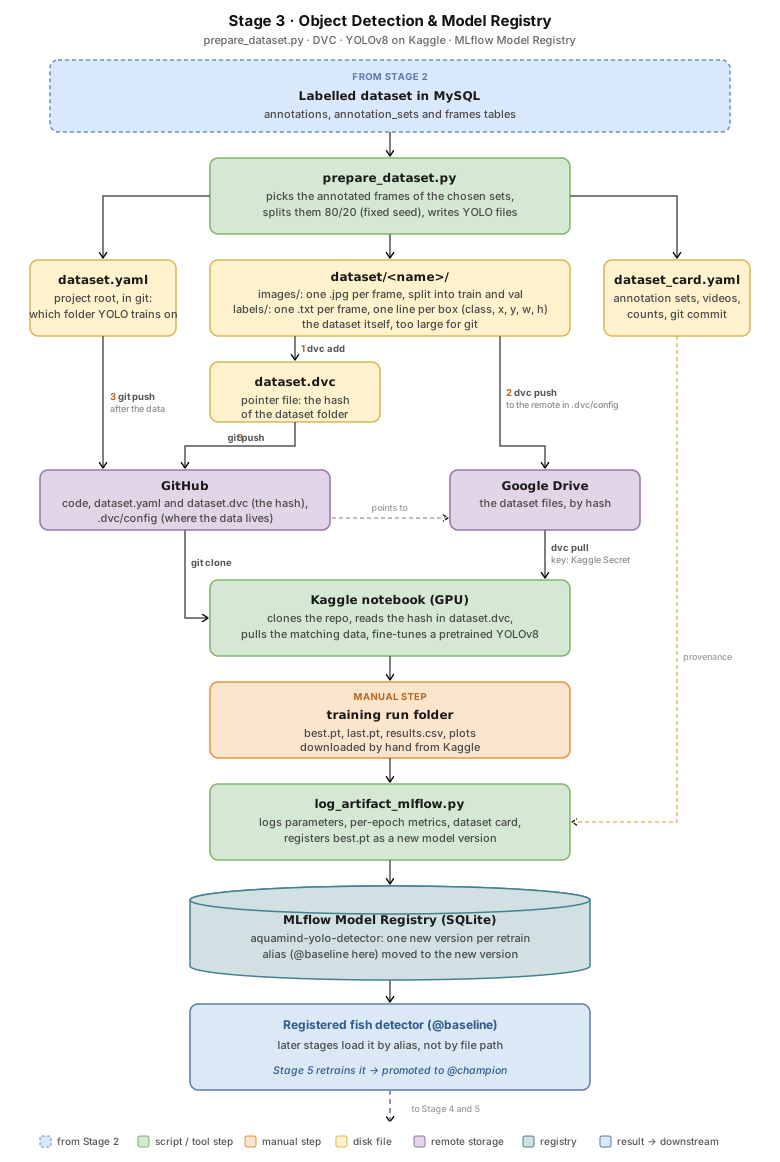
Annotated frames leave MySQL as a YOLO dataset folder, a pretrained YOLOv8 is fine-tuned on that folder on a free Kaggle GPU, and the resulting weights are registered in the MLflow Model Registry, as traced in Fig. 1 below. The subsections that follow take the pipeline step by step.

FigStage 3 pipeline: the labelled dataset from Stage 2 becomes a versioned YOLO dataset folder (prepare_dataset.py, DVC), the data travels to Google Drive and its pointer file to GitHub, a Kaggle GPU notebook brings the two back together and fine-tunes a pretrained YOLOv8, and log_artifact_mlflow.py logs the run and registers best.pt in the MLflow Model Registry, under the @baseline alias, which Stage 5 replaces with @champion. The training run is downloaded from Kaggle by hand. Click to zoom.

Building the dataset

Because the labels live in a database rather than in a single export folder, a training set is a choice rather than a fixed collection: any combination of labelling batches can be selected, and the composition becomes an experimental variable in its own right.

prepare_dataset.py (flow diagram) takes a list of annotation_set_ids from config.yaml, which is the only thing that decides what the dataset contains. Each id is one labelling batch from Stage 2: frames from one video, sampled one way, labelled together in one Label Studio project and stored as a row of annotation_sets. The script selects every distinct frame that carries at least one box from those batches, shuffles the result under a fixed random seed, and splits it 80% training and 20% validation. Splitting on frames rather than on individual boxes keeps all the boxes of a frame on the same side of the split, so the same image cannot appear in both.

Each selected frame is then copied to images/train or images/val, and its boxes are read back from annotations and written as one YOLO text file per frame in the matching labels/ folder. The split is done by seed rather than recorded, which means rebuilding the dataset from the same batch ids reproduces the same split without needing to store it.

Each box carries one of the two classes defined during labelling: danio_rerio for a real fish and reflection for its mirror image on the glass or the water surface. Reflections are kept as a trained class rather than discarded, so that the detector is shown what to reject instead of never being shown it at all.

Two small YAML files complete the folder. dataset.yaml is what YOLO itself reads: the path of the dataset and the two class names. dataset_card.yaml is for provenance and is not read by the training at all. It records the batch ids, the full metadata of every video that contributed a frame, the train and validation counts, the class map, the random seed, and the short git commit of the code that built it. That card is what makes a finished training run explicable months later, and it travels with the dataset into MLflow.

Versioning the dataset and getting it to the GPU

The dataset has to be versioned, so that each model can be traced to the exact data it learned from, and it has to reach the GPU machine where training happens. DVC (Data Version Control) does both. The dataset folder itself is too large for git, so it is tracked with DVC, a tool that works alongside git: git keeps track of the code and other small files, while DVC keeps track of large data, storing it elsewhere and leaving only a small fingerprint of it in git. dvc add computes that fingerprint, a hash of the folder’s contents, and writes it into dataset.dvc, a pointer file of a few lines. From there the data and its description travel by two separate routes, as Fig. 1 shows: dvc push uploads the dataset files to Google Drive, stored under their hash, and git push sends the code, dataset.yaml and dataset.dvc to GitHub. The hash is what ties the two together.

This matters because training does not happen on the machine that builds the dataset. The Kaggle notebook is where the two routes meet: it runs git clone to fetch the repository from GitHub, small files included, and dvc pull to fetch the data from Google Drive. Drive access goes through a Google service account whose key is never in the repository: locally it sits in a git-ignored secrets/ folder, and on Kaggle it is stored as a Kaggle Secret and written to disk only for the session. A fresh machine therefore needs nothing but the repository and that key.

Because every commit carries its own hash, running the same git clone and dvc pull on an older commit brings back the dataset as it was then. This is what lets an earlier dataset be rebuilt after a newer one has replaced it.

In short, three small files in the repository divide the work between them:

• dataset.dvc says what to fetch: the hash of the dataset.
• .dvc/config says where the data is stored: the Google Drive folder that dvc push uploads to and dvc pull downloads from.
• dataset.yaml says which folder YOLO trains on once the data is there. Its path is relative to the repository, so the same file works on the machine that built the dataset and on Kaggle, where dvc pull has rebuilt the same folder layout.

The two routes also impose an order. The data must be pushed before the pointer, or the notebook clones a hash that Google Drive cannot yet serve and dvc pull fails.

Fine-tuning the detector

The detector is built on YOLO (“You Only Look Once”), a family of object-detection models named for finding every box in an image in a single pass through the network. Like most modern detectors, it has two main parts. The backbone turns the image into visual features, from simple edges and textures in its early layers to whole shapes in its deeper ones. The head reads those features and decides where the boxes are and what each one contains.

The model used here, yolov8s (the small version of YOLOv8), was pretrained on COCO, a public dataset of everyday photographs covering 80 kinds of objects. Training on AquaMind’s frames starts from those weights rather than from random ones, which is called fine-tuning. The whole network is still trained, but its layers only need small adjustments, because what they already know about edges and shapes carries over to fish. Only the last layers of the head are new, since the model now chooses between two classes instead of eighty. The network has about 11 million parameters, the numbers adjusted during training, and when training starts, 349 of its 355 blocks of weights are copied from the pretrained model; the six that are not are the head’s class outputs, resized from 80 classes to 2. Starting from those weights is what makes training fast, and what lets a modest dataset produce a working detector.

Training runs on a free Kaggle GPU (an NVIDIA T4), in the notebook aquamind-train-yolov8.ipynb (flow diagram). It clones the repository, installs ultralytics and DVC, pulls the dataset with a Google Drive key held as a Kaggle secret rather than in the repository, and fine-tunes yolov8s for 50 epochs (full passes through the training images), with a batch size of 16 (the number of images processed together before each update of the network’s weights), on images resized to 640 pixels on their longest side. Batch size and image size are the library’s defaults. Fifty epochs was the first budget tried, and the training curves in the Results show it was enough, so it was kept.

The run’s output folder holds the best and last weights, the per-epoch metrics in results.csv, and the standard YOLO diagnostic plots. That folder is downloaded from Kaggle by hand and placed in the repository, which is the one manual link in the chain.

Logging and registering the model

MLflow serves as the project’s lab notebook for training runs. Each run is stored with the settings it was trained with, the data it saw and the scores it reached, and the MLflow web interface turns that record into something browsable: training curves drawn per run, runs compared side by side, and every plot and file one click away. Without it, the same information would sit in run folders scattered across a laptop and a Kaggle account.

log_artifact_mlflow.py (flow diagram) fills that record for one downloaded run. It logs the training parameters, the per-epoch metrics replayed from results.csv, the diagnostic plots and the whole run folder, together with the dataset card of the dataset that run trained on. The dataset name is pinned in config.yaml separately from the one prepare_dataset.py is currently building, so a run stays described by the dataset it actually saw rather than by whatever is being assembled next.

The script then registers the weights as a new version of a named model, aquamind-yolo-detector, and moves an alias to it: @baseline for this first model, @champion once Stage 5 trains a better one. Downstream code asks for models:/aquamind-yolo-detector@champion and gets whichever version the alias currently points at, so promoting a model is re-running this script rather than editing paths in several places.

Registration and loading are deliberately not symmetrical. The weights are registered through MLflow’s pyfunc interface, which wraps them in a proper model flavour so the registry holds a real model rather than a bare file, but the tracker does not load them back that way. It resolves the alias to the underlying weights and loads them with ultralytics directly, because the tracker needs the native detection API that generic pyfunc loading does not expose. The registry is used for naming and versioning, not as a serving layer.

Results

All results below are for the registered baseline, aquamind-yolo-detector version 6 (@baseline). It is a deliberate starting point, trained on ordinary frames only, and the reference that the targeted labelling of Stage 5 is measured against.

The dataset

The baseline dataset was built from three labelling batches of ordinary frames, one frame per second with no targeted selection. They come from three videos: two of five fish in a planted tank, and one of a single fish in a bare tank.

	Frames	danio_rerio boxes	reflection boxes	Total boxes
Train	208	747	374	1,121
Validation	52	178	89	267
Total	260	925	463	1,388

Reflections are a third of all boxes. The split is random per frame, so training and validation frames come from the same three videos, often a few seconds apart. The validation scores therefore measure how well the detector handles these videos, not how well it would handle a new one, and they should be read as an upper bound.

Detector performance

The weights kept are those of epoch 20, the epoch with the best validation score.

Class	Images	Boxes	Precision	Recall	mAP50	mAP50-95
danio_rerio	52	178	0.78	0.73	0.71	0.30
reflection	34	89	0.59	0.57	0.52	0.18
All	52	267	0.69	0.65	0.61	0.24

Fish are the easier class on every metric. The large gap between mAP50 and mAP50-95 says that the detector usually finds an object in roughly the right place, but its boxes are often too loose or offset to pass the stricter overlap thresholds.

FigTraining and validation curves over 50 epochs. Training losses keep falling to the end, but validation losses and all four validation metrics flatten from about epoch 15. The model stopped learning anything that transfers to the validation frames long before the 50-epoch budget ran out. Plot generated by YOLO during training.

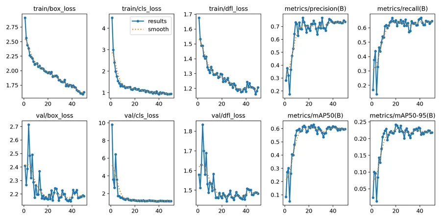
The training curves show where the limit lies. Training loss keeps falling for all 50 epochs, while validation loss and every validation metric flatten after about epoch 15. From there on the model fits its 208 training frames more closely without getting better on new ones, so more epochs would not help; more varied data would.

FigNormalised confusion matrix on the validation split. Each column is a true class. A quarter of real fish are called reflections (0.24), and a quarter of reflections are called fish (0.27). Fewer than one box in ten of either class is missed outright. Plot generated by YOLO during training.

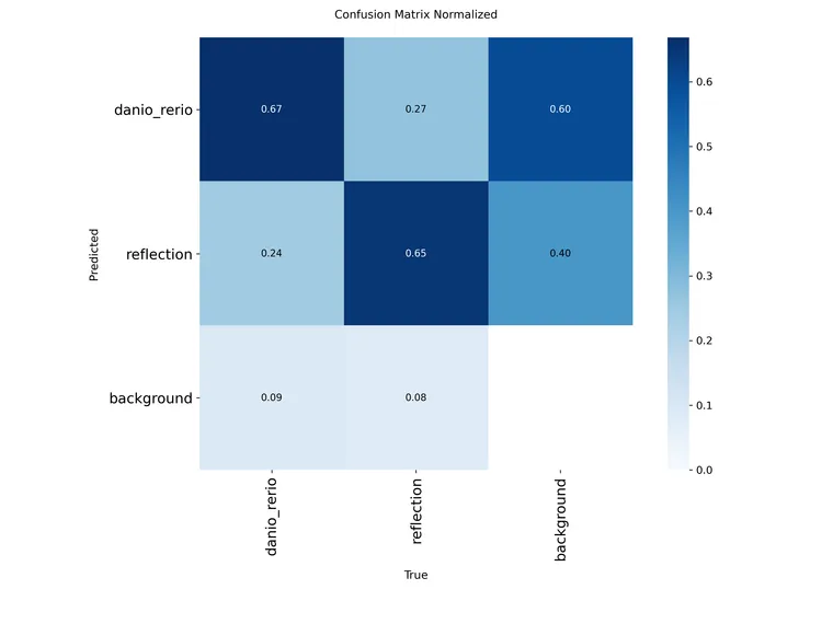
Read column by column, the main error is not missing objects but naming them wrongly. Fewer than one box in ten is missed, but 24% of real fish are detected and called reflections, and 27% of reflections are detected and called fish. Both errors matter downstream: a fish called a reflection is an animal the tracker drops, and a reflection called a fish is an animal that does not exist.

FigBaseline predictions on 16 validation frames (dark blue: fish, light blue: reflection, with confidence scores). Most fish are found, but confidences are low and the errors gather at the water surface, where a fish and its reflection sit close together. Image generated by YOLO during training.

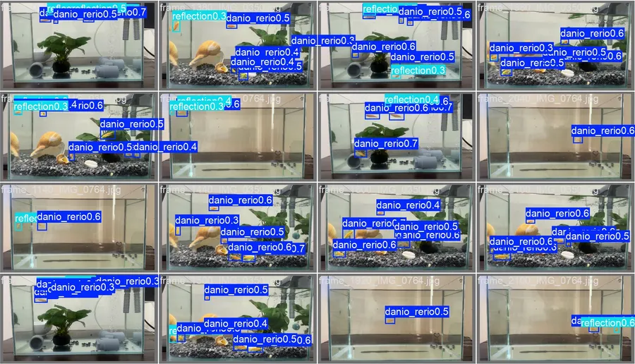
The prediction examples show where these errors happen. Most confidence scores sit between 0.3 and 0.6, so the detector is unsure even when it is right, and the mistakes gather at the water surface, where a fish swims next to its own mirror image.

Discussion

The stage set out to do two things, and the results answer them differently.

The first aim, a reproducible path from labels to a named model, was met. A dataset is now a query rather than a folder: a list of batch ids in a config file, a fixed seed, and a card that records which batches, which videos and which commit produced it. A model is a name rather than a path, and promoting a new one is re-running one script. Both held up in practice through several retraining rounds as new labelled batches arrived, which is the only real test of this kind of claim.

The second aim was to test the labelling choice made in Stage 2: does training on reflections as their own class teach the detector to tell them apart from fish? On ordinary frames alone, the answer is not yet. The detector finds nearly everything, missing fewer than one box in ten, but it names a quarter of fish as reflections (24%) and a quarter of reflections as fish (27%). It has learned that both classes exist, but not reliably which is which.

Three observations point at the data rather than the model as the cause. The validation metrics stopped improving at epoch 15 while training loss kept falling, so the run was limited by what 208 training frames could teach, not by the 50-epoch budget or the architecture. Most confidence scores sit between 0.3 and 0.6, so the detector is uncertain even when it is right. And the errors gather at the water surface, where a fish swims next to its own mirror image, a situation that is rare in frames sampled once per second. All three call for more labelled examples of the hard cases, not a bigger model or a longer schedule. That is the loop Stage 5 builds: it mines the frames where the detector fails, labels them, and retrains the same architecture, which reaches mAP50 0.85 on its own, larger validation split.

Limitations

• Optimistic validation. Training and validation frames come from the same three videos, often seconds apart, so the scores are an upper bound. A fair test of generalisation would hold out a whole video the model never trained on.
• One run, one seed. Small differences between this model and later ones are within run-to-run noise and should not be over-read.
• File-name collisions. prepare_dataset.py copies each frame under its original file name, and frames extracted in different runs of the same video can share one. The baseline is not affected (208 frames on the card, 208 on disk), but in the larger Stage 5 dataset six frames were silently overwritten, so the card says 669 training frames where 663 were written. Prefixing each copied file with its frame id would remove the collision.
• An open chain at both ends. On the way in, the notebook trains on whichever dataset the pointer file on GitHub names, so a rebuilt dataset whose new dataset.dvc was never pushed does not raise an error: the notebook quietly trains on the previous version. On the way out, the run folder is carried back by hand. Downloading it with the Kaggle command-line tool would close that second gap.
• Two MLflow backends. The registry lives in a SQLite database, while older experiments live in a file store that cannot host a registry. Nothing breaks today, but it is a seam a larger project would not tolerate.

What this stage hands on

A working baseline whose failure modes are measured rather than assumed, and a pipeline that can retrain and promote a better one in a single step. Stage 4 turns per-frame boxes into continuous tracks, where the same weakness shows up a second way: when two fish cross, the detector tends to emit one box where there are two, and the tracker has to survive it.

Reproducibility

• Code: prepare_dataset.py, aquamind-train-yolov8.ipynb, log_artifact_mlflow.py
• Model: aquamind-yolo-detector version 6 (@baseline) in the MLflow Model Registry
• Dataset: 260 frames from annotation sets 5, 9 and 10, split 80/20 with seed 42; dataset card, built at commit 9d4230a3
• Training: YOLOv8s pretrained on COCO, 50 epochs, image size 640, batch 16, training seed 0, on a Kaggle NVIDIA T4; weights kept from epoch 20
• Per-class metrics: from re-running validation on the kept weights, whose overall scores match the training log exactly